前言
本文章为《The Annotated Transformer》的学习笔记。文章名为:带有注释版的Transformer,实际上就是用代码实现了一下《attention is all your need》中的各个章节模块。原文地址:https://nlp.seas.harvard.edu/annotated-transformer/
原文是按照《attention is all your need》的章节来的。但是论文中是自顶向下,先介绍总体架构,之后再详细介绍。我打算从他的输入到输出一步步来看。
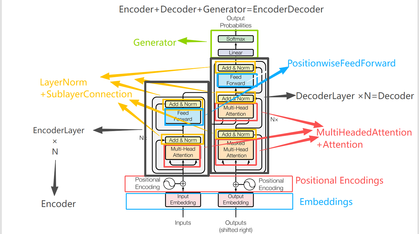
具体对应到代码中的类与模型架构图的标识如下
目录对应着每一个类或者函数
Embeddings
首先是词嵌入,这个很简单:我在前一篇文章中也解释了为什么要乘以
class Embeddings(nn.Module):
    def __init__(self, d_model, vocab):
        super(Embeddings, self).__init__()
        self.lut = nn.Embedding(vocab, d_model)#输入初始化之后会生成一个(vocab,d_model)大小的矩阵,为每一个索引生成了一个对应的向量。
        self.d_model = d_model

    def forward(self, x):
        return self.lut(x) * math.sqrt(self.d_model)
Positional Encodings
class PositionalEncoding(nn.Module):
    "Implement the PE function."

    def __init__(self, d_model, dropout, max_len=5000):
        super(PositionalEncoding, self).__init__()
        self.dropout = nn.Dropout(p=dropout)

        # Compute the positional encodings once in log space.
        pe = torch.zeros(max_len, d_model)#这里是位置编码的初始化
        #表示最多生成max_len个token生成维度为d_model的位置编码。
        position = torch.arange(0, max_len).unsqueeze(1)#(max_len,)->(max_len,1)
        div_term = torch.exp(
            torch.arange(0, d_model, 2) * -(math.log(10000.0) / d_model)
        )
        pe[:, 0::2] = torch.sin(position * div_term)
        pe[:, 1::2] = torch.cos(position * div_term)#
        pe = pe.unsqueeze(0)#(max_len, d_model)->(1,max_len, d_model)
        #
        self.register_buffer("pe", pe)#不随模型一块训练更新参数

    def forward(self, x):
        x = x + self.pe[:, : x.size(1)].requires_grad_(False)
        return self.dropout(x)
一共几个疑问:
为什么加dropout:Dropout 是深度学习中常用的正则化手段。它会随机“屏蔽”一部分神经元的输出,防止模型过拟合。embedding + PE 组成的输入向量是整个模型的基础信息多头自注意力和后续层有大量参数,如果直接全量使用 embedding,容易过拟合训练集,实际上,Transformer 里 dropout 不止这一处,后边的注意力计算,feed-forwar也会加dropout。 position = torch.arange(0, max_len).unsqueeze(1)为什么unsqueeze(1)一下,这里position就是公式里的pos,表示token的索引,这里直接先生成(0,max_len)的索引,之后要unsqueeze(1)一下,主要是让他"竖"过来:(max_len,)->(max_len,1)方便后边的计算torch.sin(position * div_term),div_term的维度为(d_model/2,),在相乘时,pytorch会自动转为:(1,d_model/2),与前面相乘,所以我们只需要unsqueeze一个即可实现计算时维度时维度匹配。
div_term = torch.exp(
           torch.arange(0, d_model, 2) * -(math.log(10000.0) / d_model)
       )
这里作者采取了一个很优雅但是可读性挺差的写法(问就是我太菜了)。
因为公式:
我们会发现两个公式只限定与i是奇数还是偶数,不管是哪个,进去之后都是。所以作者先来了一波初始化:
torch.arange(0, d_model, 2)
这一步会生成[0, 2, 4, ..., d_model-2],对应公式中的
接着给这个序列乘了一个-(math.log(10000.0) / d_model),且外边套了一个torch.exp这是为啥?
因为:
下边的记作
又因为:
所以:
所以
而在python中,math.log的底数默认为
所以
div_term = torch.exp(
           torch.arange(0, d_model, 2) * -(math.log(10000.0) / d_model)
       )
这一步就是在计算
之后
pe[:, 0::2] = torch.sin(position * div_term)
pe[:, 1::2] = torch.cos(position * div_term)
就是分别计算奇数位置和偶数位置的位置编码了。相乘之后得到的维度为:(max_len,d_model)
4. pe = pe.unsqueeze(0)将维度转为:(1,max_len,d_model)是为了满足和x相加,因为文字编码向量维度为:(batch_size,seq_len,d_model)
5. self.register_buffer("pe", pe)的作用是把 pe 注册成一个 buffer,而不是 nn.Parameter,nn.Parameter → 会被认为是模型的 可训练参数,会参与反向传播和梯度更新。register_buffer → 注册成 buffer,会随模型一起保存/加载(比如 state_dict),但不会更新梯度。因为位置编码是个固定函数(正弦余弦),不需要训练,但我们又希望它能随着模型一起保存,所以用 buffer
6.
x = x + self.pe[:, : x.size(1)].requires_grad_(False)
因为pe的维度为:(1,max_len,d_model),而x为(batch_size,seq_len,d_model),这里就是取出seq_len长度的位置编码,要和x对齐,之后就可以利用pytorch的广播机制,将第一维自动对齐再相加。
而requires_grad_(False)的作用是告诉pytorch:这些张量在反向传播时不要算梯度.
而如何将embedding和Positional Encodings结合在一起呢?
源码里是利用了nn.Sequential将他俩连在一起:
c = copy.deepcopy
position = PositionalEncoding(d_model, dropout)
nn.Sequential(Embeddings(d_model, src_vocab), c(position)),
nn.Sequential(Embeddings(d_model, tgt_vocab), c(position)),
深拷贝的作用:
layer = nn.Linear(10, 20)
net = nn.Sequential(layer, layer)
那么这两个位置 实际上用的是同一个层对象,共享参数。→ 前向传播的时候,两次调用都会用到 同一套权重。有时候我们想复用逻辑,但希望每次调用有 独立的权重。这时候就需要 copy.deepcopy。
这里之所以深拷贝一下是为了保险,实际上他俩共享权重也是没什么的。因为位置编码都不进行更新,共享不共享也没什么了。
Attention
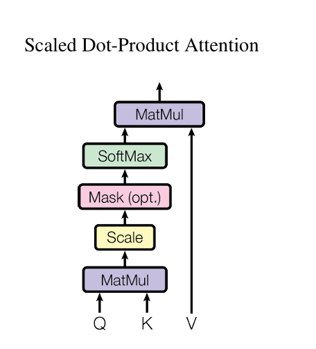
论文中的注意力计算方式为:
代码为:
def attention(query, key, value, mask=None, dropout=None):
    "Compute 'Scaled Dot Product Attention'"
    d_k = query.size(-1)
    scores = torch.matmul(query, key.transpose(-2, -1)) / math.sqrt(d_k)
    if mask is not None:
        scores = scores.masked_fill(mask == 0, -1e9)
    p_attn = scores.softmax(dim=-1)
    if dropout is not None:
        p_attn = dropout(p_attn)
    return torch.matmul(p_attn, value), p_attn
首先我们要知道,该函数是要在后边的多头注意力函数中使用,所以我们传进来的query、向量维度为(batch_size,head_num,seqlen_q,d_k),key维度为(batch_size,head_num,seqlen_k,d_k)而value的序列长度和key相同,所以value维度为(batch_size,head_num,seqlen_k,d_v)。
所以第一行先取了,然后,第二行就是计算缩放点积注意力分数,torch.matmul为矩阵乘法,因为是计算,所以需要将key矩阵转置,将Key向量倒数第二维和倒数第一维transpose一下。,然后除以
masked_fill()函数详解
然后需要理解一下的就是这个mask操作
if mask is not None:
        scores = scores.masked_fill(mask == 0, -1e9)
首先看torch.Tensor.masked_fill()这个函数,他的输入有两个,一个是BoolTensor,另一个是value,他的意思就是将BoolTensor中为false的地方设置为value。
在此例子中,scores是和相乘得到的,那么维度就为(batch_size,head_num,seqlen_q,seqlen_k)。那对应的mask_tensor的维度就应该为(batch_size,1,seqlen_q,seqlen_k),第二维可以通过广播机制对齐。
虽然官方文档中写的masked_fill的第一个参数需要一个BoolTensor,但实际上经过我的测试,true,false,或者直接1,0矩阵都可以。
import torch

scores=torch.tensor([[1.0,2.0,3.0],[4.0,5.0,6.0]])
mask=torch.tensor([[1,0,1],[0,1,1]])
# mask=mask.bool()
print(mask)
scores = scores.masked_fill(mask==0, 666)
print(scores)
输出为:
tensor([[1, 0, 1],
        [0, 1, 1]])
tensor([[  1., 666.,   3.],
        [666.,   5.,   6.]])
意味着将对应mask张量中为0的地方设置为value,而当代码为:
import torch

scores=torch.tensor([[1.0,2.0,3.0],[4.0,5.0,6.0]])
mask=torch.tensor([[1,0,1],[0,1,1]])
# mask=mask.bool()
print(mask)
scores = scores.masked_fill(mask, 666)
print(scores)
或者:
import torch

scores=torch.tensor([[1.0,2.0,3.0],[4.0,5.0,6.0]])
mask=torch.tensor([[1,0,1],[0,1,1]])
# mask=mask.bool()
print(mask)
scores = scores.masked_fill(mask==1, 666)
print(scores)
上边两种的输出都是:,可以看到如果不标明,会将mask张量中为1的地方设置为value
tensor([[1, 0, 1],
        [0, 1, 1]])
tensor([[666.,   2., 666.],
        [  4., 666., 666.]])
而当输入boolTensor时,
import torch

scores=torch.tensor([[1.0,2.0,3.0],[4.0,5.0,6.0]])
mask=torch.tensor([[1,0,1],[0,1,1]])
mask=mask.bool()
print(mask)
scores = scores.masked_fill(mask, 666)
print(scores)
结果为:
tensor([[ True, False,  True],
        [False,  True,  True]])
tensor([[666.,   2., 666.],
        [  4., 666., 666.]])
以上都是关于masked_fill()函数的实验,现在我们已经知道这个函数是如何工作的了。
之后的代码:
p_attn = scores.softmax(dim=-1)
    if dropout is not None:
        p_attn = dropout(p_attn)
    return torch.matmul(p_attn, value), p_attn
scores的最后一维就是对到的注意力分数。p_attn = scores.softmax(dim=-1)这一步就是对最后一维softmax一下,得到权重分布。这里的p_attn维度为:(batch_size,head_num,seq_len_q,seq_len_k),而value的维度为(batch_size,head_num,seq_len_v,d_v)而一般K和V是来自同一个序列,所以seq_k==seq_v所以最终得到的维度为(batch_size,head_num,seq_len_q,d_v),而transforer中,d_k和d_v是相同的,所以最终的维度也为:(batch_size,head_num,seq_len_q,d_k)
当然如果计算的是自注意力,那么QKV的seq_len都是相同的,但是在transformer中有一种情况是decoder中的q,以及encoder中的k,v。
MultiHeadedAttention
首先是init函数
class MultiHeadedAttention(nn.Module):
    def __init__(self, h, d_model, dropout=0.1):
        "Take in model size and number of heads."
        super(MultiHeadedAttention, self).__init__()
        assert d_model % h == 0
        # We assume d_v always equals d_k
        self.d_k = d_model // h
        self.h = h
        self.linears = clones(nn.Linear(d_model, d_model), 4)
        self.attn = None #注意力分数,后边需要通过attention函数计算
        self.dropout = nn.Dropout(p=dropout)
前几行没什么好说的,第一个看不懂的是这行:
self.linears = clones(nn.Linear(d_model, d_model), 4)
这个clone函数得去开头的encoder中找,定义为:
def clones(module, N):
    "Produce N identical layers."
    return nn.ModuleList([copy.deepcopy(module) for _ in range(N)])
这个nn.ModouleList直接看官方文档就行:
ModuleList can be indexed like a regular Python list, but modules it contains are properly registered, and will be visible by all Module methods.
class MyModule(nn.Module):
    def __init__(self) -> None:
        super().__init__()
        self.linears = nn.ModuleList([nn.Linear(10, 10) for i in range(10)])

    def forward(self, x):
        # ModuleList can act as an iterable, or be indexed using ints
        for i, l in enumerate(self.linears):
            x = self.linears[i // 2](x) + l(x)
        return x
而我们的clones函数就是生成N个相同的module,且是deepcopy的,即都是相互独立的权重。
所以:
self.linears = clones(nn.Linear(d_model, d_model), 4)
这行代码就是生成4个线性层,且是d_model到d_model的线性变换。每个线性层的权重矩阵大小为(d_model,d_model),是可训练的。至于他是干什么的,需要看下边的forward函数。
 def forward(self, query, key, value, mask=None):
        "Implements Figure 2"
        if mask is not None:
            # Same mask applied to all h heads.
            mask = mask.unsqueeze(1)
        nbatches = query.size(0)#batch_size

        # 1) Do all the linear projections in batch from d_model => h x d_k
        query, key, value = [
            lin(x).view(nbatches, -1, self.h, self.d_k).transpose(1, 2)
            for lin, x in zip(self.linears, (query, key, value))
        ]

        # 2) Apply attention on all the projected vectors in batch.
        x, self.attn = attention(
            query, key, value, mask=mask, dropout=self.dropout
        )

        # 3) "Concat" using a view and apply a final linear.
        x = (
            x.transpose(1, 2)
            .contiguous()
            .view(nbatches, -1, self.h * self.d_k)
        )
        del query
        del key
        del value
        return self.linears[-1](x)
从输入上来看:query,key,value函数的张量大小都为:(batch_size,seq_len,d_model)。如果是自注意力,则seq_len相同,否则就像上边说的一样,query是单独的长度,key和value是一个长度。
mask = mask.unsqueeze(1),mask输入进来的大小为:(batch_size,seq_len_q,seq_len_k)。这里注释也说了:Same mask applied to all h heads.对于所有头都使用一个mask,所以需要unsqueeze一下给他加一个维度,变成(batch_size,1,seq_len_q,seq_len_k)其中第二维对应head_num。
接着就是这行代码:
 query, key, value = [
            lin(x).view(nbatches, -1, self.h, self.d_k).transpose(1, 2)
            for lin, x in zip(self.linears, (query, key, value))
        ]
这个做的其实就是将QKV分别放到每个多头注意力中的每个头中,对应论文中就是:。其中。但这里有个疑问,为什么linear是d_model映射到d_model而不是变成d_k。是因为我们做的针对于一个大矩阵的。
在代码中,先经过线性层,之后又做了一个view操作,将张量reshape成:(batch_size,seq_len,head_num,d_k)大小。之后transpose了一下,变成成(batch_size,head_num,seq_len,d_k)(因为后边的attention函数的输入就是这样的维度)。
这一步我们既有线性变换,有可训练的参数矩阵,又实现了Do all the linear projections in batch from d_model => h x d_k。
所以很多时候公式和代码是有区别的,代码为了实现并行运算,都会将数据放到大的矩阵中。
然后是:
x, self.attn = attention(
            query, key, value, mask=mask, dropout=self.dropout
        )
经过上边的attention函数,得到了包含注意力信息的V向量,以及每个token对其他token的注意力分数self.attn。
最后是concat操作
x = ( x.transpose(1, 2) .contiguous() .view(nbatches, -1, self.h * self.d_k) )
前面得到的x的维度为:(batch_size,head_num,seq_len_q,d_v)
我们还记得前面的代码是:
lin(x).view(nbatches, -1, self.h, self.d_k).transpose(1, 2)
因为原始的x维度是:(batch_size,seq_len,d_model) 而 d_model=head_num*d_k 所以我们view必须是将self.h, self.d_k放到后边两个维度,以便于拆分。同理,现在我们要concat回去,所以也需要将head_num和d_k放到后边,所以这一步transpose就是将(batche_size,head_num,seq_len_q,d_v)其中(d_k==d_v)变成
(batche_size,seq_len_q,head_num,d_v),之后再.contiguous()一下,这个函数的作用是将transpose之后生成的view在内存中重新排列,保证内存连续,因为view()函数需要内存连续。
这样我们就重新将函数拼接为(batch_size,seq_len,d_model)大小了
最后:return self.linears[-1](x),即再次经过一个线性层。
经过这个我们发现,这些分头,拼接的操作,在原论文中都是使用权重矩阵来线性变换转换维度大小的,而在代码实现中,我们的线性变换并没有将他维度转换,而是不变,之后通过.view函数进行转换。
LayerNorm
经过MultiHeadedAttention之后,就到了add&Norm层,这层有两个功能:残差连接+layerNorm.首先来看LayerNorm的实现:
class LayerNorm(nn.Module):
    "Construct a layernorm module (See citation for details)."

    def __init__(self, features, eps=1e-6):
        super(LayerNorm, self).__init__()
        self.a_2 = nn.Parameter(torch.ones(features))
        self.b_2 = nn.Parameter(torch.zeros(features))
        self.eps = eps

    def forward(self, x):
        mean = x.mean(-1, keepdim=True)
        std = x.std(-1, keepdim=True)
        return self.a_2 * (x - mean) / (std + self.eps) + self.b_2
LayerNorm就是对一个样本(一个序列)中的所有值(token)进行归一化,
首先我们需要看一下此函数使用的归一化函数的数学定义:
实际上即使减去均值,除以标准差,之后线性映射,其中是防止分母为0。既然都线性映射了,那么和都是可训练的参数。
所以初始化函数中:
self.a_2 = nn.Parameter(torch.ones(features))
self.b_2 = nn.Parameter(torch.zeros(features))
就是对和的初始化,nn.Parameter的作用就是将该tensor变成可训练的参数,PyTorch 会自动把它加入 model.parameters(),训练时会被优化器更新。
其中,输入features一般和d_model的大小一样。
所以在forward函数中:
def forward(self, x):
        mean = x.mean(-1, keepdim=True)
        std = x.std(-1, keepdim=True)
        return self.a_2 * (x - mean) / (std + self.eps) + self.b_2
输入x的大小为:(batch_size,seq_len,d_model)
我们所有的操作都是对最后一维的token内部的向量做归一化。
SublayerConnection
然后是残差连接
class SublayerConnection(nn.Module):
    """
    A residual connection followed by a layer norm.
    Note for code simplicity the norm is first as opposed to last.
    """

    def __init__(self, size, dropout):
        super(SublayerConnection, self).__init__()
        self.norm = LayerNorm(size)
        self.dropout = nn.Dropout(dropout)

    def forward(self, x, sublayer):
        "Apply residual connection to any sublayer with the same size."
        return x + self.dropout(sublayer(self.norm(x)))
总体很简单,这里有两个需要注意的地方,
forward函数需要传入的参数sublayer,他代表MultiHeadedAttention或者FeedForward。 代码里使用的是先将输入LN之后,再进行残差连接,而原论文中是,即先进行残差连接再归一化。这里的理由在注释中写道:Note for code simplicity the norm is first as opposed to last.作者的理由是为了代码simple一些,选择先归一化再残差连接,并且还把归一化放到了Sublayer前面,而不是先过子层,再进行归一化。
所以代码是return x + self.dropout(sublayer(self.norm(x)))而不是return x + self.dropout(self.norm(sublayer(x)))
这样的做法有利于训练更稳定,梯度容易流动。
PositionwiseFeedForward
这里接着向下走就是FeedForward部分,这部分很简单,就是两个线性层,
class PositionwiseFeedForward(nn.Module):
    "Implements FFN equation."

    def __init__(self, d_model, d_ff, dropout=0.1):
        super(PositionwiseFeedForward, self).__init__()
        self.w_1 = nn.Linear(d_model, d_ff)
        self.w_2 = nn.Linear(d_ff, d_model)
        self.dropout = nn.Dropout(dropout)

    def forward(self, x):
        return self.w_2(self.dropout(self.w_1(x).relu()))
EncoderLayer
前面这些层完事之后,就可以看一下整个的encoder了。
class EncoderLayer(nn.Module):
    "Encoder is made up of self-attn and feed forward (defined below)"

    def __init__(self, size, self_attn, feed_forward, dropout):
        super(EncoderLayer, self).__init__()
        self.self_attn = self_attn
        self.feed_forward = feed_forward
        self.sublayer = clones(SublayerConnection(size, dropout), 2)
        self.size = size

    def forward(self, x, mask):
        "Follow Figure 1 (left) for connections."
        x = self.sublayer[0](x, lambda x: self.self_attn(x, x, x, mask))
        return self.sublayer[1](x, self.feed_forward)
这么看有点莫名奇妙,从字面意思不太能理解size, self_attn, feed_forward都是什么,我们先来看一下调用该类的地方:
    c = copy.deepcopy
    attn = MultiHeadedAttention(h, d_model)
    ff = PositionwiseFeedForward(d_model, d_ff, dropout)
    position = PositionalEncoding(d_model, dropout)
    model = EncoderDecoder(
        Encoder(EncoderLayer(d_model, c(attn), c(ff), dropout), N),
        Decoder(DecoderLayer(d_model, c(attn), c(attn), c(ff), dropout), N),
        nn.Sequential(Embeddings(d_model, src_vocab), c(position)),
        nn.Sequential(Embeddings(d_model, tgt_vocab), c(position)),
        Generator(d_model, tgt_vocab),
    )
可以看到size就是d_model,而self_attn, feed_forward分别指MultiHeadedAttention、FeedForward这两层。
self.sublayer = clones(SublayerConnection(size, dropout), 2)
然后我们clone了两层SublayerConnection,用来连接。
最后就是forward函数了,
x = self.sublayer[0](x, lambda x: self.self_attn(x, x, x, mask))
return self.sublayer[1](x, self.feed_forward)
SublayerConnection的forwa函数需要传入x和Sublayer函数,这里的Sublayer函数是MultiHeadedAttention,即self.self_attn(),这个函数需要传的参数为(query,key,value,mask)。这里是直接传进了三个x,这里也是纠正了我之前的误区。
原论文中:
他这个下边的三个Q,K,V应该是三个x,但这个就很容易让人认为这个QKV是x经过了线性变换的结果。实际上只有一次线性变换。所以这是我之前一直有的一个误区。
然后还有一个问题:为什么用lambda x:而不是直接像下边的feed_forward这样self.self_attn(x, x, x, mask)。因为self.sublayer[0]是SublayerConnection,而他的前向传播为:
 def forward(self, x, sublayer):
        return x + self.dropout(sublayer(self.norm(x)))
sublayer需要是一个只传一个参数的函数,而self.self_attn是三个,所以需要给他封装一下。
Encoder
接着是Encoder的实现
class Encoder(nn.Module):
    "Core encoder is a stack of N layers"

    def __init__(self, layer, N):
        super(Encoder, self).__init__()
        self.layers = clones(layer, N)
        self.norm = LayerNorm(layer.size)

    def forward(self, x, mask):
        "Pass the input (and mask) through each layer in turn."
        for layer in self.layers:
            x = layer(x, mask)
        return self.norm(x)
老样子还是看看这个类是怎么定义的:
    model = EncoderDecoder(
        Encoder(EncoderLayer(d_model, c(attn), c(ff), dropout), N),
        Decoder(DecoderLayer(d_model, c(attn), c(attn), c(ff), dropout), N),
        nn.Sequential(Embeddings(d_model, src_vocab), c(position)),
        nn.Sequential(Embeddings(d_model, tgt_vocab), c(position)),
        Generator(d_model, tgt_vocab),
    )
所以初始化函数中的layer即为上一节的EncoderLayer,N就是几层,在原论文中,作者用了6层,所以N默认就是6。
self.layers = clones(layer, N)
        self.norm = LayerNorm(layer.size)
然后就是clones 6层,之后来一个层归一化。
forward函数也非常简单,就是简单的堆叠,最后加一个LN。
DecoderLayer
因为encoder和decoder两个类很多模块都是相同的。所以直接看DecoderLayer
class DecoderLayer(nn.Module):
    "Decoder is made of self-attn, src-attn, and feed forward (defined below)"

    def __init__(self, size, self_attn, src_attn, feed_forward, dropout):
        super(DecoderLayer, self).__init__()
        self.size = size
        self.self_attn = self_attn
        self.src_attn = src_attn
        self.feed_forward = feed_forward
        self.sublayer = clones(SublayerConnection(size, dropout), 3)
首先看init,和encoderLayer基本差不多,但多了一个参数:src_attn,我们很自然的可以想到,这应该就是decoder中的那个非自注意力:即用target seq的Q和source seq的K和V来计算注意力分数以及结果。其他的都和encoder一样。
    def forward(self, x, memory, src_mask, tgt_mask):
        "Follow Figure 1 (right) for connections."
        m = memory
        x = self.sublayer[0](x, lambda x: self.self_attn(x, x, x, tgt_mask))
        x = self.sublayer[1](x, lambda x: self.src_attn(x, m, m, src_mask))
        return self.sublayer[2](x, self.feed_forward)
然后是forward函数,多了三个和之前不同的参数:
memory, src_mask, tgt_mask
首先看memory,在后边它的作用是
x = self.sublayer[1](x, lambda x: self.src_attn(x, m, m, src_mask))
通过这个代码我们可以推断出memory是什么,他是来自encoder的输出,是架构中的交叉注意力部分。
然后是src_mask和tgt_mask。这是两种不同的mask。通过名字也可以推断出他们的mask作用,tgt_mask就是针对目标序列的掩码,即经过decoder架构中的第一个mask,该mask属于因果编码(subsequent mask),是为了屏蔽未来的位置,他是一个上三角矩阵。
而src_mask就和前面encoderlayer中的那个mask一样了,属于padding mask(填充掩码):屏蔽序列末尾的 <PAD> token,不让模型注意填充位。
实际上,这两个mask的生成方式文中也都有。
其中tgt_mask的生成方式为:
class Batch:
    """Object for holding a batch of data with mask during training."""

    def __init__(self, src, tgt=None, pad=2):  # 2 = <blank>
        self.src = src
        self.src_mask = (src != pad).unsqueeze(-2)
        if tgt is not None:
            self.tgt = tgt[:, :-1]
            self.tgt_y = tgt[:, 1:]
            self.tgt_mask = self.make_std_mask(self.tgt, pad)
            self.ntokens = (self.tgt_y != pad).data.sum()

    @staticmethod
    def make_std_mask(tgt, pad):
        "Create a mask to hide padding and future words."
        tgt_mask = (tgt != pad).unsqueeze(-2)
        tgt_mask = tgt_mask & subsequent_mask(tgt.size(-1)).type_as(
            tgt_mask.data
        )
        return tgt_mask
def subsequent_mask(size):
    "Mask out subsequent positions."
    attn_shape = (1, size, size)
    subsequent_mask = torch.triu(torch.ones(attn_shape), diagonal=1).type(
        torch.uint8
    )
    return subsequent_mask == 0
可以看到self.src_mask = (src != pad).unsqueeze(-2),这里src是索引序列而不是embedding,而这里用2指代<PAD>,所以(src != pad)的意义是:在src中,不等于pad(pad==2)的地方设置为True,表示不屏蔽,
这里src的形状为:(batch_size,src_len),.unsqueeze(-2)表示在倒数第二维插入一个维度 → 变为 (batch, 1, src_len),因为在MultiHeadedAttention()函数中,与(batch, heads, seq_q, d_k)维度的张量对齐。
而self.tgt_mask = self.make_std_mask(self.tgt, pad)
在make_std_mask函数中,先是进行了和src一样的处理来屏蔽pad,然后subsequent_mask的作用是用来生成用于屏蔽未来word的mask矩阵,即下三角为True,上三角为false的矩阵,之后再和已经根据<PAD>生成的mask按位&一下(padding mask会自动广播对齐),其中.type_as(tgt_mask.data)表示统一二者的单位,否则一个为int变量,一个为bool变量,不能进行计算,最终得到最终的tgt_mask就是既包含subsequent mask又包含padding mask。
其他的具体细节后边在介绍batch的时候详细介绍。
Decoder
class Decoder(nn.Module):
    "Generic N layer decoder with masking."

    def __init__(self, layer, N):
        super(Decoder, self).__init__()
        self.layers = clones(layer, N)
        self.norm = LayerNorm(layer.size)

    def forward(self, x, memory, src_mask, tgt_mask):
        for layer in self.layers:
            x = layer(x, memory, src_mask, tgt_mask)
        return self.norm(x)
基本和encoder代码差不多。没什么好说的
Generator
现在架构中只有一个部分没有说明了,那就是从decoder中出来之后,经过的Linear和softmax,Generator类就是实现这个的
class Generator(nn.Module):
    "Define standard linear + softmax generation step."

    def __init__(self, d_model, vocab):
        super(Generator, self).__init__()
        self.proj = nn.Linear(d_model, vocab)

    def forward(self, x):
        return log_softmax(self.proj(x), dim=-1)
vocab就是词表大小,将d_model大小的张量映射到vocab大小,来形成对每一个词的打分,之后经过log_softmax,来对最后一个维度进行打分并转换成概率分布
x的维度变换为:(batch_size,seq_len,d_model)--->(batch_size,seq_len,vocab)
这里用log_softmax的原因:
在后边的训练中,作者使用的损失函数为:nn.KLDivLoss,input输入要求为:log probability,所以这里用的是log_softmax。
EncoderDecoder
最后就是将上边提到的这些类封装起来的最大的一个类了。
首先是init函数
class EncoderDecoder(nn.Module):
    """
    A standard Encoder-Decoder architecture. Base for this and many
    other models.
    """

    def __init__(self, encoder, decoder, src_embed, tgt_embed, generator):
        super(EncoderDecoder, self).__init__()
        self.encoder = encoder
        self.decoder = decoder
        self.src_embed = src_embed
        self.tgt_embed = tgt_embed
        self.generator = generator
要想看懂init,必须先去看看怎么用它的:
    c = copy.deepcopy
    attn = MultiHeadedAttention(h, d_model)
    ff = PositionwiseFeedForward(d_model, d_ff, dropout)
    position = PositionalEncoding(d_model, dropout)
    model = EncoderDecoder(
        Encoder(EncoderLayer(d_model, c(attn), c(ff), dropout), N),
        Decoder(DecoderLayer(d_model, c(attn), c(attn), c(ff), dropout), N),
        nn.Sequential(Embeddings(d_model, src_vocab), c(position)),
        nn.Sequential(Embeddings(d_model, tgt_vocab), c(position)),
        Generator(d_model, tgt_vocab),
    )
可以看到,就是将我们上边讲到的类封装了一下。最重要的还是看看他的其他函数:
    def forward(self, src, tgt, src_mask, tgt_mask):
        "Take in and process masked src and target sequences."
        return self.decode(self.encode(src, src_mask), src_mask, tgt, tgt_mask)

    def encode(self, src, src_mask):
        return self.encoder(self.src_embed(src), src_mask)

    def decode(self, memory, src_mask, tgt, tgt_mask):
        return self.decoder(self.tgt_embed(tgt), memory, src_mask, tgt_mask)
forward函数的输入为src, tgt, src_mask, tgt_mask,这里的src和tgt都为为索引序列
forward就是先经过encode,再将encode的输出作为输入放到decode中,最后输出。
可以看到这个类中唯一没有用到的属性是self.generator。这个属性主要是在后边训练的时候用到的。
make_model
最后就是如何创建模型了,一般简单的模型,就直接通过model=Mymodel()这样的形式。但这个模型蛮大的,虽然说最后封装到EncoderDecoder中了,但是Encoder和Decoder都需要MultiHeadedAttention()和PositionwiseFeedForward()。但他们必须是独立的参数,所以需要deepcopy,再然后如果将所有参数都写到model=EncoderDecoder()中,就未免太臃肿了。所以单独写了一个make_model函数来再次封装,用来创建模型
def make_model(
    src_vocab, tgt_vocab, N=6, d_model=512, d_ff=2048, h=8, dropout=0.1
):
    "Helper: Construct a model from hyperparameters."
    c = copy.deepcopy
    attn = MultiHeadedAttention(h, d_model)
    ff = PositionwiseFeedForward(d_model, d_ff, dropout)
    position = PositionalEncoding(d_model, dropout)
    model = EncoderDecoder(
        Encoder(EncoderLayer(d_model, c(attn), c(ff), dropout), N),
        Decoder(DecoderLayer(d_model, c(attn), c(attn), c(ff), dropout), N),
        nn.Sequential(Embeddings(d_model, src_vocab), c(position)),
        nn.Sequential(Embeddings(d_model, tgt_vocab), c(position)),
        Generator(d_model, tgt_vocab),
    )

    # This was important from their code.
    # Initialize parameters with Glorot / fan_avg.
    for p in model.parameters():
        if p.dim() > 1:
            nn.init.xavier_uniform_(p)
    return model
实际上我们在前面也多次提到这段代码了,copy.deepcopy的作用就是使每层EncoderLayer以及DecoderLayer独立使用一份MultiHeadedAttention 和 PositionwiseFeedForward,每层都有自己单独的权重。实际上position不需要copy,因为位置编码是不变的,但作者可能为了看起来整齐也给加上了一层copy。
然后就是权重初始化
for p in model.parameters():
        if p.dim() > 1:
            nn.init.xavier_uniform_(p)
这段代码将维度大于1的参数,也就是权重矩阵,使用xavier初始化。
推理测试
在文章中:
Here we make a forward step to generate a prediction of the model. We try to use our transformer to memorize the input. As you will see the output is randomly generated due to the fact that the model is not trained yet. In the next tutorial we will build the training function and try to train our model to memorize the numbers from 1 to 10.
这里作者写了一个函数来测试推理,让模型来推理下一个词为1到10的哪个,当然,模型没有经过训练,输出的都是随机的。
def inference_test():
    test_model = make_model(11, 11, 2)
    test_model.eval()
    src = torch.LongTensor([[1, 2, 3, 4, 5, 6, 7, 8, 9, 10]])
    src_mask = torch.ones(1, 1, 10)

    memory = test_model.encode(src, src_mask)
    ys = torch.zeros(1, 1).type_as(src)

    for i in range(9):
        out = test_model.decode(
            memory, src_mask, ys, subsequent_mask(ys.size(1)).type_as(src)
        )
        prob = test_model.generator(out[:, -1])
        # print(prob)
        _, next_word = torch.max(prob, dim=1)#返回最大值和最大值所在的索引,我们只需要索引
        print(next_word)
        next_word = next_word[0]
        ys = torch.cat(
            [ys, torch.empty(1, 1).type_as(src).fill_(next_word)], dim=1
        )

    print("Example Untrained Model Prediction:", ys)


def run_tests():
    for _ in range(10):
        inference_test()
src为输入序列,可以看到只是一个1到10的longtensor,维度为(1,10)。因为是推理,所以batch设置为1,针对一个样本,然后seqlen为10,src_mask也是直接全1,表示在encoder中不mask,维度为(batche_size,1,seq_len),然后在attention函数中,mask = mask.unsqueeze(1)变成(batch_size,1,1,seqlen),方便广播对其多头注意力中计算attention时的维度:(batch_size,head_num,seq_len,seq_len)
然后ys 为生成序列,这里初始化让第一个元素为0,表示<BOS>,之后就是在for i in range(9)不断的生成下一个word。
其中:
# 生成上三角为False的矩阵, 即subsequent mask
def subsequent_mask(size):
    "Mask out subsequent positions."
    attn_shape = (1, size, size)
    subsequent_mask = torch.triu(torch.ones(attn_shape), diagonal=1).bool() #会生成上三角为True的矩阵

    return subsequent_mask ==False  #取反,使得上三角为False
也是利用了torch.triu生成subsequent mask,在调用的时候我们传入的是ys.size(1),ys是当前生成序列,形状 (batch, tgt_len),tgt_len = 当前已经生成的 token 数(包括起始 token),所以传入ys.size(1)生成tgt_len大小的上三角为False的矩阵,表示屏蔽i后边个的word.
未完待续
到这里整个的Model_Architecture都就结束了,
这次再看一下这个类分布图就会清晰一些。
本文主要是介绍了一下模型怎么搭的,作者的码风还是太优雅了,有些地方直接看真的看不太懂。下一章打算学习一下怎么训练这个模型。