本文最后更新于 934 天前,其中的信息可能已经有所发展或是发生改变。
数据集选用鸢尾花数据集,并且为了方便画图,选取其中两个特征进行训练分类。
数据处理
In [1]:
import pandas as pd
import numpy as np
from sklearn.datasets import load_iris
import matplotlib.pyplot as plt

%matplotlib inline
#无需调用plt.show()
选用鸢尾花数据集,并且只取其中的两个特征进行分析(方便画图)
In [2]:
# load data
iris = load_iris()
df = pd.DataFrame(iris.data, columns=iris.feature_names)
df['label'] = iris.target
df
Out[2]:
| sepal length (cm) | sepal width (cm) | petal length (cm) | petal width (cm) | label | |
|---|---|---|---|---|---|
| 0 | 5.1 | 3.5 | 1.4 | 0.2 | 0 |
| 1 | 4.9 | 3.0 | 1.4 | 0.2 | 0 |
| 2 | 4.7 | 3.2 | 1.3 | 0.2 | 0 |
| 3 | 4.6 | 3.1 | 1.5 | 0.2 | 0 |
| 4 | 5.0 | 3.6 | 1.4 | 0.2 | 0 |
| ... | ... | ... | ... | ... | ... |
| 145 | 6.7 | 3.0 | 5.2 | 2.3 | 2 |
| 146 | 6.3 | 2.5 | 5.0 | 1.9 | 2 |
| 147 | 6.5 | 3.0 | 5.2 | 2.0 | 2 |
| 148 | 6.2 | 3.4 | 5.4 | 2.3 | 2 |
| 149 | 5.9 | 3.0 | 5.1 | 1.8 | 2 |
150 rows × 5 columns
In [3]:
df.columns = [
    'sepal length', 'sepal width', 'petal length', 'petal width', 'label'
]
df.label.value_counts()
Out[3]:
0    50
1    50
2    50
Name: label, dtype: int64
In [4]:
plt.scatter(df[:50]['sepal length'], df[:50]['sepal width'], label='0')
plt.scatter(df[50:100]['sepal length'], df[50:100]['sepal width'], label='1')

plt.xlabel('sepal length')
plt.ylabel('sepal width')
plt.legend()
Out[4]:
<matplotlib.legend.Legend at 0x1ab2500a550>

In [5]:
data = np.array(df.iloc[:100, [0, 1, -1]])
X_t, y_t = data[:,:-1], data[:,-1]
y_t = np.array([1 if i == 1 else -1 for i in y_t])
感知机的一般形式
In [6]:
# 数据线性可分,二分类数据
# 此处为一元一次线性方程
class Model:
    def __init__(self):
        #初始化权重值w、偏执、学习率
        self.w = np.zeros(len(data[0])-1, dtype=np.float32)
        self.b = 0
        self.l_rate = 0.1
        # self.data = data

    def sign(self, x, w, b):
        y = np.dot(x, w) + b
       # print(y)
        #这里本质上就是判断他是正是负,所以其实不用判断这一步,如果手算的话,转化成-1和+1比较好算,课本上也是这样的,所以就这里转化一下。
        return 1 if y>=0 else -1 #sign函数 如果大于等于0就返回1,否则返回-1

    # 随机梯度下降法
    def fit(self, X_train, y_train):
        is_wrong = False
        train_num=0
        while not is_wrong:#这里因为数据是线性可分的,所以没有设置迭代次数
            train_num+=1
            wrong_count = 0
            for d in range(len(X_train)):
                X = X_train[d]
                y = y_train[d]
                #更新参数
                if y * self.sign(X, self.w, self.b) <= 0:
                    self.w = self.w + self.l_rate*np.dot(y, X)
                    self.b = self.b + self.l_rate*y
                    wrong_count += 1
            if wrong_count == 0:
                is_wrong = True
        print("w:{},b:{}".format(self.w,self.b))#训练完成的w和b
        return '训练完成,迭代{}次'.format(train_num)

    def score(self):
        pass
In [7]:
perceptron = Model()
perceptron.fit(X_t, y_t)
w:[ 7.9 -10.07],b:-12.399999999999972
Out[7]:
'训练完成,迭代701次'
In [8]:
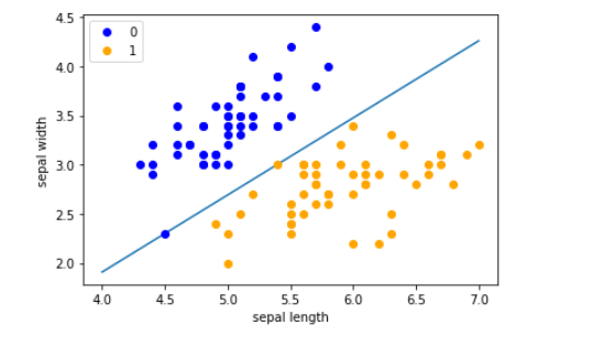
x_points = np.linspace(4, 7,10)#因为上边的数据集的特征都分布在大概4 到 7 这个范围
#得到的线是:w0*x0+w1*x1+b=0,
x1 = -(perceptron.w[0]*x_points + perceptron.b)/perceptron.w[1] #纵坐标是特征值x1,
plt.plot(x_points, x1)

plt.plot(data[:50, 0], data[:50, 1], 'o', color='blue', label='0')
plt.plot(data[50:100, 0], data[50:100, 1], 'o', color='orange', label='1')
plt.xlabel('sepal length')
plt.ylabel('sepal width')
plt.legend()
Out[8]:
<matplotlib.legend.Legend at 0x1ab2575cc70>

感知机的对偶形式
In [9]:
class dual_Model():

    def __init__(self, eta=1, n_iter=10):
        self.eta=eta
        self.alpha, self.Gram_matrix = None, None
        self.n_iter=n_iter

    def fit(self, X_train, Y_train):
        n_samples, dim = X_train.shape
        self.alpha, self.w, self.b = np.zeros(n_samples), np.zeros(dim), 0
        # Gram matrix
        self.Gram_matrix = np.dot(X_train, X_train.T)
        train_num=0
        # Iteration
        i = 0
        while i < n_samples:
            #
            wx = np.sum(np.dot(self.Gram_matrix[i, :] , self.alpha * Y_train))

            if Y_train[i] * (wx + self.b) <= 0:
                # a <- a + eta, b <- b + eta * y_i
                self.alpha[i] += self.eta
                self.b += self.eta * Y_train[i]
                i = 0
            else:
                i += 1
            train_num+=1

        print(f'迭代次数:{train_num}')
        self.w = np.sum(X_train * np.tile((self.alpha * Y_train).reshape((n_samples, 1)), (1, dim)), axis=0)
In [10]:
dualperceptron = dual_Model()
dualperceptron.fit(X_t, y_t)
print(f'w:{dualperceptron.w},b:{dualperceptron.b}')
迭代次数:67813
w:[  78.2 -100.4],b:-121
In [11]:
x_points = np.linspace(4, 7,10)#因为上边的数据集的特征都分布在大概4 到 7 这个范围
#得到的线是:w0*x0+w1*x1+b=0,
x1 = -(dualperceptron.w[0]*x_points + dualperceptron.b)/dualperceptron.w[1] #纵坐标是特征值x1,
plt.plot(x_points, x1)

plt.plot(data[:50, 0], data[:50, 1], 'o', color='blue', label='0')
plt.plot(data[50:100, 0], data[50:100, 1], 'o', color='orange', label='1')
plt.xlabel('sepal length')
plt.ylabel('sepal width')
plt.legend()
Out[11]:
<matplotlib.legend.Legend at 0x1ab25895100>

sklearn 实现
In [79]:
from sklearn.linear_model import Perceptron
clf = Perceptron()
clf.fit(X_t, y_t)
Out[79]:
Perceptron()
In [80]:
print(clf.coef_,clf.intercept_)# w和b的值
[[ 23.2 -38.7]] [-5.]
In [81]:
x_points = np.linspace(4, 7,10)#因为上边的数据集的特征都分布在大概4 到 7 这个范围
#得到的线是:w0*x0+w1*x1+b=0,
x1 = -(clf.coef_[0][0]*x_points + clf.intercept_)/clf.coef_[0][1] #纵坐标是特征值x1,
plt.plot(x_points, x1)

plt.plot(data[:50, 0], data[:50, 1], 'o', color='blue', label='0')
plt.plot(data[50:100, 0], data[50:100, 1], 'o', color='orange', label='1')
plt.xlabel('sepal length')
plt.ylabel('sepal width')
plt.legend()
Out[81]:
<matplotlib.legend.Legend at 0x1ab279f10a0>

In [ ]:
In [ ]: